A | B | C | D | E | F | G | H | CH | I | J | K | L | M | N | O | P | Q | R | S | T | U | V | W | X | Y | Z | 0 | 1 | 2 | 3 | 4 | 5 | 6 | 7 | 8 | 9
You can help expand this article with text translated from the corresponding article in German. (September 2019) Click for important translation instructions.
|


In statistics, the coefficient of determination, denoted R2 or r2 and pronounced "R squared", is the proportion of the variation in the dependent variable that is predictable from the independent variable(s).
It is a statistic used in the context of statistical models whose main purpose is either the prediction of future outcomes or the testing of hypotheses, on the basis of other related information. It provides a measure of how well observed outcomes are replicated by the model, based on the proportion of total variation of outcomes explained by the model.[1][2][3]
There are several definitions of R2 that are only sometimes equivalent. One class of such cases includes that of simple linear regression where r2 is used instead of R2. When only an intercept is included, then r2 is simply the square of the sample correlation coefficient (i.e., r) between the observed outcomes and the observed predictor values.[4] If additional regressors are included, R2 is the square of the coefficient of multiple correlation. In both such cases, the coefficient of determination normally ranges from 0 to 1.
There are cases where R2 can yield negative values. This can arise when the predictions that are being compared to the corresponding outcomes have not been derived from a model-fitting procedure using those data. Even if a model-fitting procedure has been used, R2 may still be negative, for example when linear regression is conducted without including an intercept,[5] or when a non-linear function is used to fit the data.[6] In cases where negative values arise, the mean of the data provides a better fit to the outcomes than do the fitted function values, according to this particular criterion.
The coefficient of determination can be more (intuitively) informative than MAE, MAPE, MSE, and RMSE in regression analysis evaluation, as the former can be expressed as a percentage, whereas the latter measures have arbitrary ranges. It also proved more robust for poor fits compared to SMAPE on the test datasets in the article.[7]
When evaluating the goodness-of-fit of simulated (Ypred) vs. measured (Yobs) values, it is not appropriate to base this on the R2 of the linear regression (i.e., Yobs= m·Ypred + b).[citation needed] The R2 quantifies the degree of any linear correlation between Yobs and Ypred, while for the goodness-of-fit evaluation only one specific linear correlation should be taken into consideration: Yobs = 1·Ypred + 0 (i.e., the 1:1 line).[8][9]
Definitionsedit

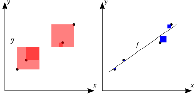
The better the linear regression (on the right) fits the data in comparison to the simple average (on the left graph), the closer the value of R2 is to 1. The areas of the blue squares represent the squared residuals with respect to the linear regression. The areas of the red squares represent the squared residuals with respect to the average value.
A data set has n values marked y1, ..., yn (collectively known as yi or as a vector y = y1, ..., ynT), each associated with a fitted (or modeled, or predicted) value f1, ..., fn (known as fi, or sometimes ŷi, as a vector f).
Define the residuals as ei = yi − fi (forming a vector e).
If is the mean of the observed data:
- The sum of squares of residuals, also called the residual sum of squares:
- The total sum of squares (proportional to the variance of the data):
The most general definition of the coefficient of determination is
In the best case, the modeled values exactly match the observed values, which results in and R2 = 1. A baseline model, which always predicts y, will have R2 = 0. Models that have worse predictions than this baseline will have a negative R2.
Relation to unexplained varianceedit
In a general form, R2 can be seen to be related to the fraction of variance unexplained (FVU), since the second term compares the unexplained variance (variance of the model's errors) with the total variance (of the data):
As explained varianceedit
A larger value of R2 implies a more successful regression model.[4]: 463 Suppose R2 = 0.49. This implies that 49% of the variability of the dependent variable in the data set has been accounted for, and the remaining 51% of the variability is still unaccounted for. For regression models, the regression sum of squares, also called the explained sum of squares, is defined as
In some cases, as in simple linear regression, the total sum of squares equals the sum of the two other sums of squares defined above:
See Partitioning in the general OLS model for a derivation of this result for one case where the relation holds. When this relation does hold, the above definition of R2 is equivalent to
where n is the number of observations (cases) on the variables.
In this form R2 is expressed as the ratio of the explained variance (variance of the model's predictions, which is SSreg / n) to the total variance (sample variance of the dependent variable, which is SStot / n).
This partition of the sum of squares holds for instance when the model values ƒi have been obtained by linear regression. A milder sufficient condition reads as follows: The model has the form
where the qi are arbitrary values that may or may not depend on i or on other free parameters (the common choice qi = xi is just one special case), and the coefficient estimates and are obtained by minimizing the residual sum of squares.
This set of conditions is an important one and it has a number of implications for the properties of the fitted residuals and the modelled values. In particular, under these conditions:
As squared correlation coefficientedit
In linear least squares multiple regression with an estimated intercept term, R2 equals the square of the Pearson correlation coefficient between the observed and modeled (predicted) data values of the dependent variable.
In a linear least squares regression with a single explanator but without an intercept term, this is also equal to the squared Pearson correlation coefficient of the dependent variable and explanatory variable
It should not be confused with the correlation coefficient between two explanatory variables, defined as
Antropológia
Aplikované vedy
Bibliometria
Dejiny vedy
Encyklopédie
Filozofia vedy
Forenzné vedy
Humanitné vedy
Knižničná veda
Kryogenika
Kryptológia
Kulturológia
Literárna veda
Medzidisciplinárne oblasti
Metódy kvantitatívnej analýzy
Metavedy
Metodika
Text je dostupný za podmienok Creative
Commons Attribution/Share-Alike License 3.0 Unported; prípadne za ďalších
podmienok.
Podrobnejšie informácie nájdete na stránke Podmienky
použitia.
www.astronomia.sk | www.biologia.sk | www.botanika.sk | www.dejiny.sk | www.economy.sk | www.elektrotechnika.sk | www.estetika.sk | www.farmakologia.sk | www.filozofia.sk | Fyzika | www.futurologia.sk | www.genetika.sk | www.chemia.sk | www.lingvistika.sk | www.politologia.sk | www.psychologia.sk | www.sexuologia.sk | www.sociologia.sk | www.veda.sk I www.zoologia.sk


